youll learn how to use the LEFT function in Excel.
The LEFT function is used to return the first character or characters present in the cell, based on the number that we specify in the formula.
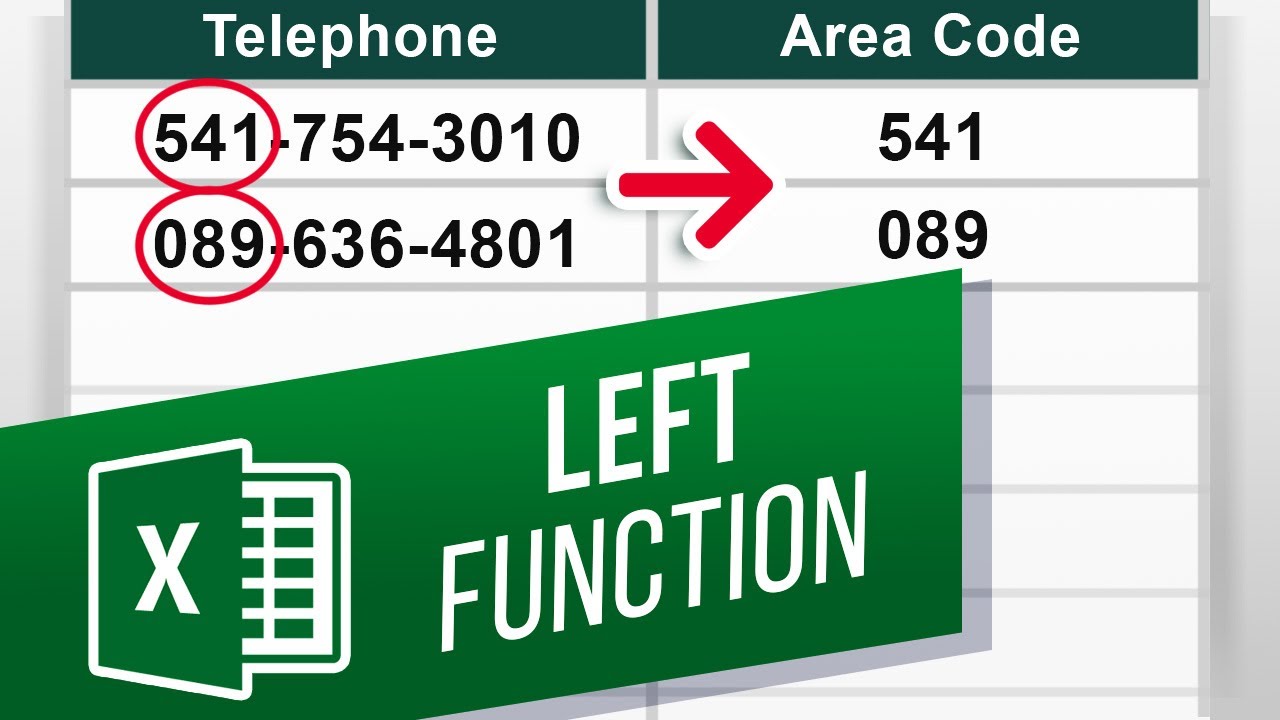
Over here, we have an employee sheet with telephone numbers in one column. Numbers in the column include area codes as well, and a standard is followed throughout the sheet. Now lets say we want to show only the area codes in a different column?
Instead of manually typing in the first three characters in the cell for each row, we would use the LEFT function and copy it throughout the sheet.
So lets select the column where we want to insert the function and enter the equals to key. After that, lets type LEFT followed by an open bracket. Now, we would be required to select the cell that contains the characters we want extracted. So, lets move the cursor and select the cell with the telephone number.
If you simply hit enter, this function returns only the first character by default. Therefore, lets specify the number of characters we want the LEFT function to extract.
Lets double click on the cell to open the function edit mode. After the cell selection here, lets enter a comma and type 3. This would return the first three characters in the cell, which in this case is the area code.
Hit enter, and you can see that the LEFT function has extracted the first three characters from the cell.
Now you can move the cursor to the corner of the cell, and when the cursor changes, simply double click to copy and paste the function to the entire sheet Date: 2023-07-08